MPC controller made easy

CasADi MPC Controller

# python # optimization # control # programming

tl;dr

The second most popular controller out there is the Model Predictive Control (MPC) controller, there is an unbelieveable number of variations around this controller, e.g, Data-driven MPC, Robust MPC, Nonlinear MPC. At the time of this writing, we can see MPC often beating Reinforcement Learning approaches in many tasks. In general, the hard part of this controller is to come up with a resilient model of the plant.

There are many examples in the real-world that are fit to a controller, and many jobs require to design such a controller.

Design a valve to ensure the engine temperature lies in the desired range.
Adjust the interest rate of central banks according to Taylor’s rule.
Design a cruise controller to ensure safety and minimal fuel use for autonomous trucks.
Design an artificial pancreas to regulate the amount of produced insulin when a high level of sugar in the bloodstream is detected and keep it within an optimal range.

The list could go on forever, but it’s obvious designing controllers is a key part of engineering and societies. Ideally, you could tackle each one of them with MPC but it’s not always the right tool to address every problem. Before MPC, Proportional-Integral-Derivative (PID) controller was “the” controller as it doesn’t depend on a mathematical model, which means nonlinearities are not a problem, and it has three knobs to adjust the controller — one for each component. Of course, it has many disadvantages, and again it does not work for complex tasks; it can even can be cumbersome to set up for engineers for systems with multiple inputs and multiple outputs.

Optimization

An MPC controller is presented as an optimization problem. You have an objective function or functional $J$ , which you want to minimize over certain variables, subject to given constraints. The name of this optimization problem is Constrained linear-quadratic optimal control and it is defined as follows.

\begin{aligned} \min_{\substack{u_0, \dots ,u_{k-1} \\ x_0, \dots ,x_k}} \quad & \sum^{k-1}_{k=0} \left(x^T_k Q x_k + u^T_k R u_k\right) + x^T_k S x_k \\ \textrm{s.t.} \quad & x_{k+1} = A x_k + B u_k \ \text{for} \ k = 0, \dots ,k-1\\ & x_0 = X_0 \\ & x_k \in \mathcal{X}_k \\ & u_k \in \mathcal{U}_k \end{aligned}

This above is a linear MPC controller as the dynamics represented by the first constraint is a state-space model with matrices $(A, B)$ . If the system in question is nonlinear in its dynamics, then it can be simply be formulated like this instead.

\begin{aligned} \min_{\substack{u_0, \dots ,u_{k-1} \\ x_0, \dots ,x_k}} \quad & \sum^{k-1}_{k=0} \left(x^T_k Q x_k + u^T_k R u_k\right) + x^T_k S x_k \\ \textrm{s.t.} \quad & x_{k+1} = f(x_k, u_k) \ \text{for} \ k = 0, \dots ,k-1\\ & x_0 = X_0 \\ & x_k \in \mathcal{X}_k \\ & u_k \in \mathcal{U}_k \end{aligned}

Where we replace the linear state-space model for a nonlinear function $f$ with the same arguments. There are nuances in order to come up with $x_k = f(x_k, u_k)$ equation, but I’ll explain it further into the reading.

CasADi implementation

It’s worth starting to introduce CasADi, which is an open-source project aiming to solve nonlinear optimization problems, and dedicated for algorithmic differentiation. It’s super nice because it’s available for Octave/Matlab, Python, and C++. In here, I’ll be showing the Python implementation.

The API at first may seem a bit overwhelming and it takes a while to grasp the documentation and finally coming out with a well-written solution. CasADi has various ways of implementing a given problem, but I’ve found that the Opti stack — introduced in Release 3.3.0 — is the best and most straightforward way of implementing and solving optimization problems like the ones we’re discussing.

Rosenbrock Problem

The Rosenbrock problem is likely the most popular optimization problem out there given its form and works as a benchmark for solvers.

\begin{aligned} \min_{x, y} \quad & (1 - x)^2 + (y - x^2)^2 \\ \textrm{s.t.} \quad & x^2 + y^2 = 1 \\ & y \geq x \\ \end{aligned}

In CasADi, it’s super simple to implement, thanks to Opti stack.

import casadi

opti = casadi.Opti()

x = opti.variable()
y = opti.variable()

opti.minimize((1 - x)^2 + (y - x^2)^2)
opti.subject_to(x^2 + y^2 == 1)
opti.subject_to(y >= x)

opti.solver('ipopt')
sol = opti.solve()

print(sol.value(x))
print(sol.value(y))

Solvers

CasADi can interface with multiple NLP solvers, but the most popular one is Interior Point Optimization (IPOPT) which comes out-of-the-box. Other solvers must be installed first such as SNOPT, WORHP, and KNITRO; it also applies for QP solvers.

An MPC application

In robotics, autonomous wheeled robots have always been of great interest, and nowadays the perfect example is self-driving cars. However, we won’t delve into the controls of a full-fledge car because it can get really nasty in terms of complexity, so we’ll apply this to simple theoretical models.

The unicycle model

The most basic model is the unicycle model.

It’s a single wheel that can rollover its footprint and can rotate around its vertical axis. Obviously, it cannot move sideways like any normal wheel would not do. There are exceptions but in this case, we’ll just work with this nonholonomic system. So here are the kinematics of such system.

\begin{cases} \dot{x} = v \cos \theta \\ \dot{y} = v \sin \theta \\ \dot{\theta} = \omega \end{cases}

It’s a nonlinear system of differential equations where the state variables are $(x, y, \theta)$ , and the input are $(v, \omega)$ . If you take a closer look, you will see that this can be reduced to a simple expression, given that we create these other two variables $\mathbf{x} = \begin{bmatrix} x & y & \theta \end{bmatrix}^T$ and $\mathbf{u} = \begin{bmatrix} v & \omega \end{bmatrix}^T$ .

\dot{\mathbf{x}} = f(\mathbf{x}, \mathbf{u})

Basically, it’s just notation but so that it’s clear that we can use this in the MPC problem! There are systems that do not come in this form right off the bat and we need to wrestle with those a bit more.

Point Stabilization

The first trivial task is to make this vehicle reach a point and stay there. The assumptions we’re making to approach this task are:

The domain, terrain or plane on which the vehicle operates is convex, meaning that vehicle can reach the target point by following a straight line.
There are no obstacles on the terrain, which is basically derived by the domain being convex.
No external forces interact with the vehicle, e.g, wind forces, wheel friction.

Use import casasdi as ca to use CasADi API.

So the first thing we must do is the define the vehicle kinematics to use it with our controller, and even simulate it, and ultimately plotting it.

def unicycle_kinematics(x, u):
    theta = x[2]
    v = u[0]
    omega = u[1]

    # return a casadi vector, be careful with
    # numpy interoperatibility
    return ca.vertcat(
        v * ca.cos(theta),
        v * ca.sin(theta),
        omega,
    )

At this point, we going to just set up the MPC problem, we won’t run it yet.

N = 20  # running horizon
num_states = 3  # length of the state vector
num_inputs = 2  # length of the input vector

opti = ca.Opti()
x = opti.variable(num_states, N + 1)
u = opti.variable(num_inputs, N)
x0 = opti.parameter(num_states)
r = opti.parameter(num_states)

There are a couple things we did above. First and foremost, defining the horizon N with which we’ll work with. Then, the a couple of variables to use that’ll help us define our opti variables. The variable x, and u are two opti.variable that CasADi will use to compute the solution on every timestep. On top of that, we need parameters; x0 that is considered the initial state at each timestep and the reference. The latter will just be used to define the target our vehicle needs to reach. Recall it’s the final state that our state vector needs to reach.

After that is settled, we need to start thinking about our objective function J. As defined previously, our cost function is a quadratic function comprised of matrices Q and R in this case. These matrices are important because they’ll be our knobs to tune the controller so it meets our expected criteria.

Lastly, we need to symbolically compute the objective function, and set the first natural constraint; next, add it to the optimizer.

J = 0  # objective function

f = unicycle_kinematics  # transition function

Q = np.diag([1.0, 5.0, 0.1])  # state weighing matrix
R = np.diag([0.5, 0.05])  # controls weighing matrix

dt = 0.2

for k in range(N):
    J += (x[:, k] - r).T @ Q @ (x[:, k] - r) + u[:, k].T @ R @ u[:, k]
    x_next = x[:, k] + f(x[:, k], u[:, k]) * dt
    opti.subject_to(x[:, k + 1] == x_next)

opti.minimize(J)

One thing to note is that the since unicycle_kinematics is a nonlinear function that’s described in continuous time, it must be discretized using the forward Euler method. It’s not the only way we could do this.

x_{k+1} = x_k + f(x_k, u_k) \Delta t

If you print(J) you will not get a value, but rather Python objects representing the sym objective function.

Now we add more constraints to limit the control input as well as specifying that first value of the horizon must be equal to the initial state. This initial state when we run it will keep changing.

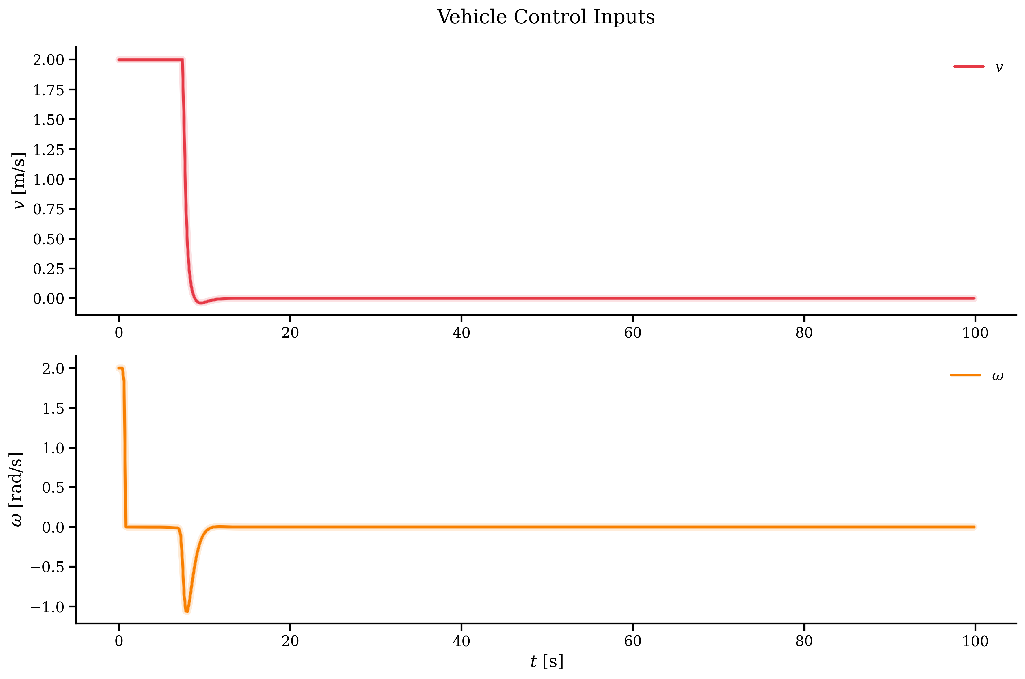
opti.subject_to(x[:, 0] == x0)
opti.subject_to(u[0, :] >= -2)
opti.subject_to(u[0, :] <= 2)
opti.subject_to(u[1, :] >= -2)
opti.subject_to(u[1, :] <= 2)

We’re close, we just now need to set the very first initial state and the target state vector, the reference in this case. Also, a bit of configuration for the solver, not too important right now.

opti.set_value(x0, ca.vertcat(0, 0, 0))
opti.set_value(r, ca.vertcat(1.5, 15, 0))

p_opts = {
    "expand": True,
}
s_opts = {
    "max_iter": 1000,
    "print_level": 0,
    "acceptable_tol": 1e-8,
    "acceptable_obj_change_tol": 1e-6,
}

opti.solver("ipopt", p_opts, s_opts)

The rest is easy, we’re going to keep track of all the x and u values while running the simulation, as well as the error. The breaking condition of the loop can be achieved if: a) the target has been reached, b) the simulation time has expired.

In each timestep, we need to update x0, which is super important because the vehicle has moved and reach some point in space and we need to run the solver again but at this time the intial position is different.

The last important part is actually passing the computed control input to the system. In this case, since it’s a mathematically simulated model, we run the kinematics with the computed input, and keep the value. If you’re actually driving a vehicle either in a 3D simulated environment or in the real world, this part has to be replaced by sending the control cue in a different way.

k = 0
T = 100

x_history = np.zeros((num_states, int(T / dt)))
u_history = np.zeros((num_inputs, int(T / dt)))
error_history = np.zeros((num_states, int(T / dt)))

start = time.time()
x_current = opti.value(x0)
while np.linalg.norm(x_current - opti.value(r)) > 1e-3 and k < T / dt:
    inner_start = time.time()

    error = np.linalg.norm(x_current - opti.value(r))

    error_history[:, k] = np.linalg.norm(
        x_current.reshape(-1, 1) - opti.value(r).reshape(-1, 1),
        axis=1,
    )

    print(f"Step = {k} Timestep = {k * dt:.2f} Error = {error:.4f}")

    sol = opti.solve()
    u_opt = sol.value(u)
    x_history[:, k] = x_current
    u_history[:, k] = u_opt[:, 0]

    x_current += f(x_current, u_opt[:, 0]).full().flatten() * dt

    opti.set_value(x0, x_current)

    k += 1

    print(f"MPC time step: {(time.time() - inner_start):.4f}")

print(f"Total MPC time: {(time.time() - start):.2f}")

The results out of all of this can be plotted. The trajectory and the position of the vehicle per component, showing that it reaches the goal in around 10 seconds and then the controller keeps it there.

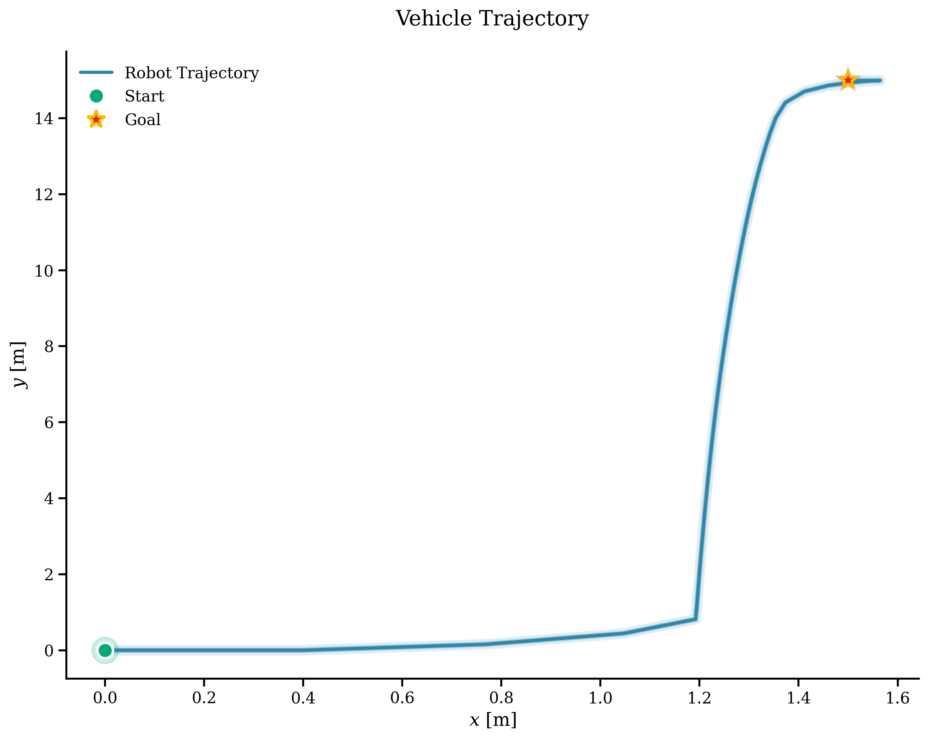
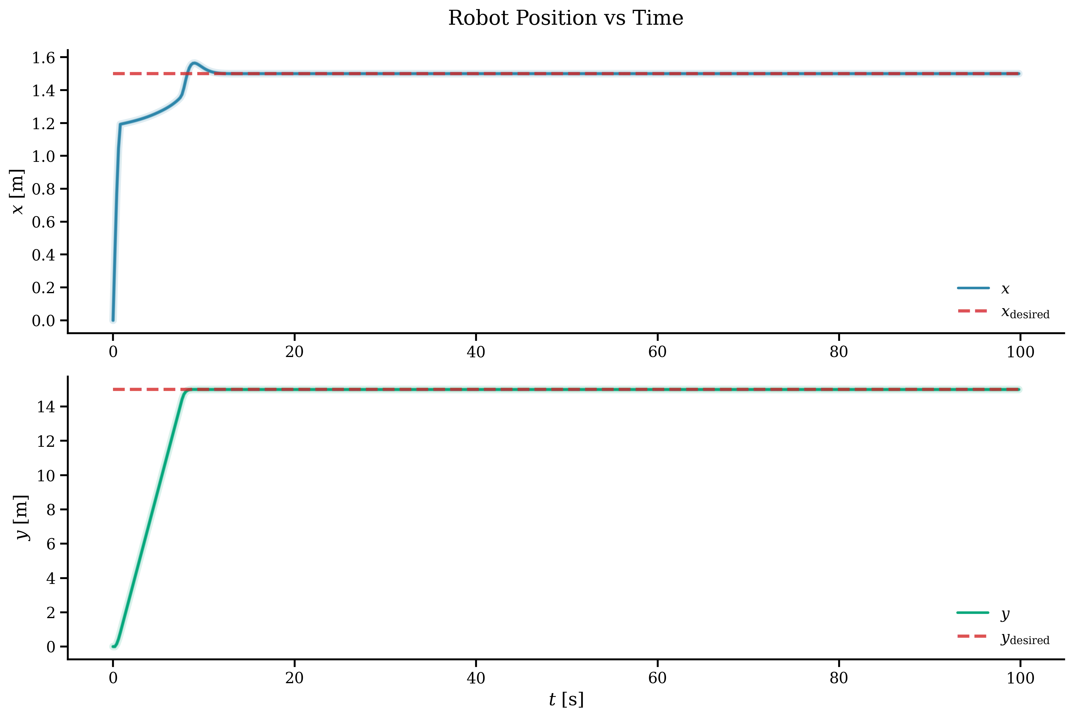
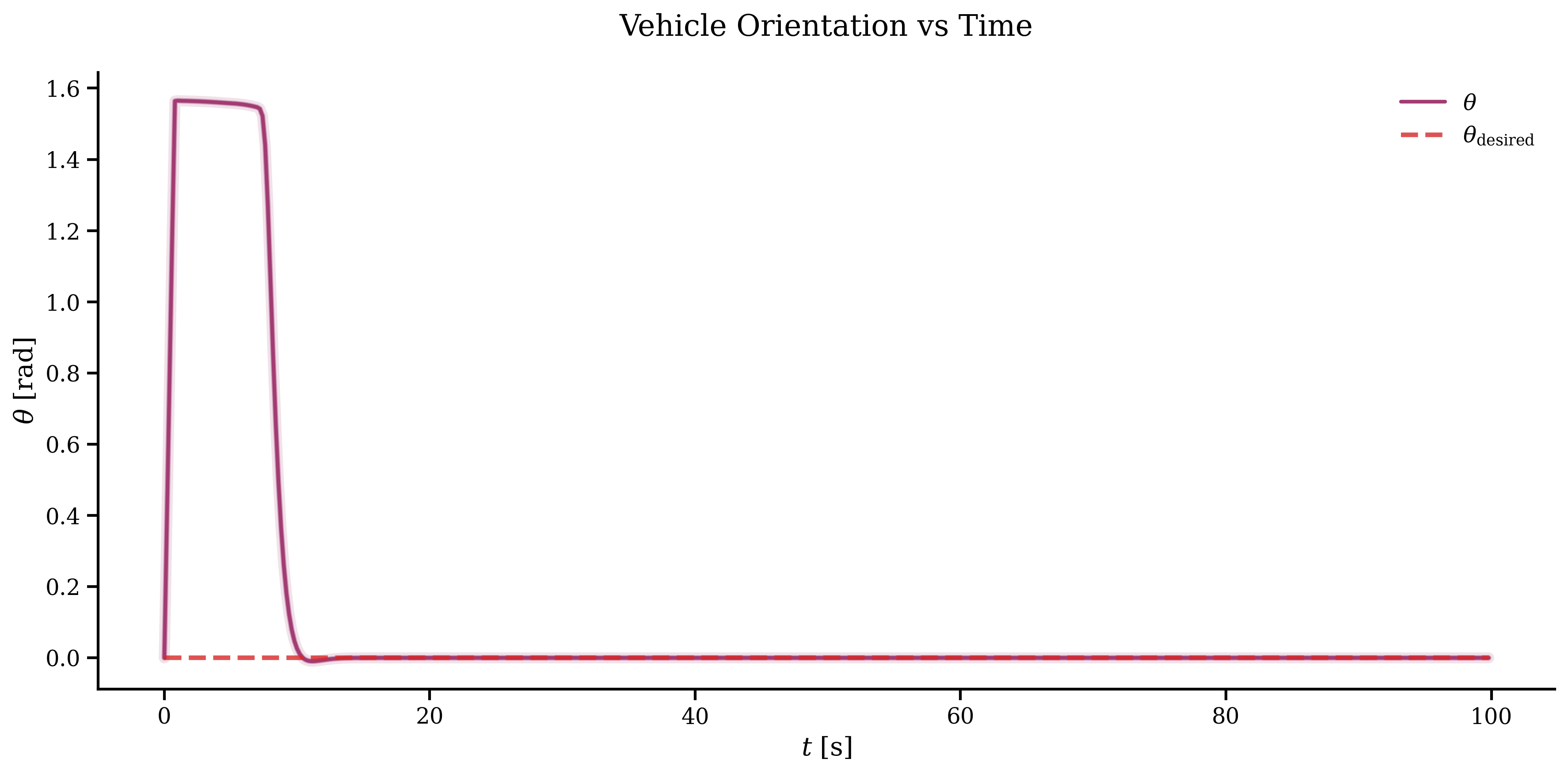
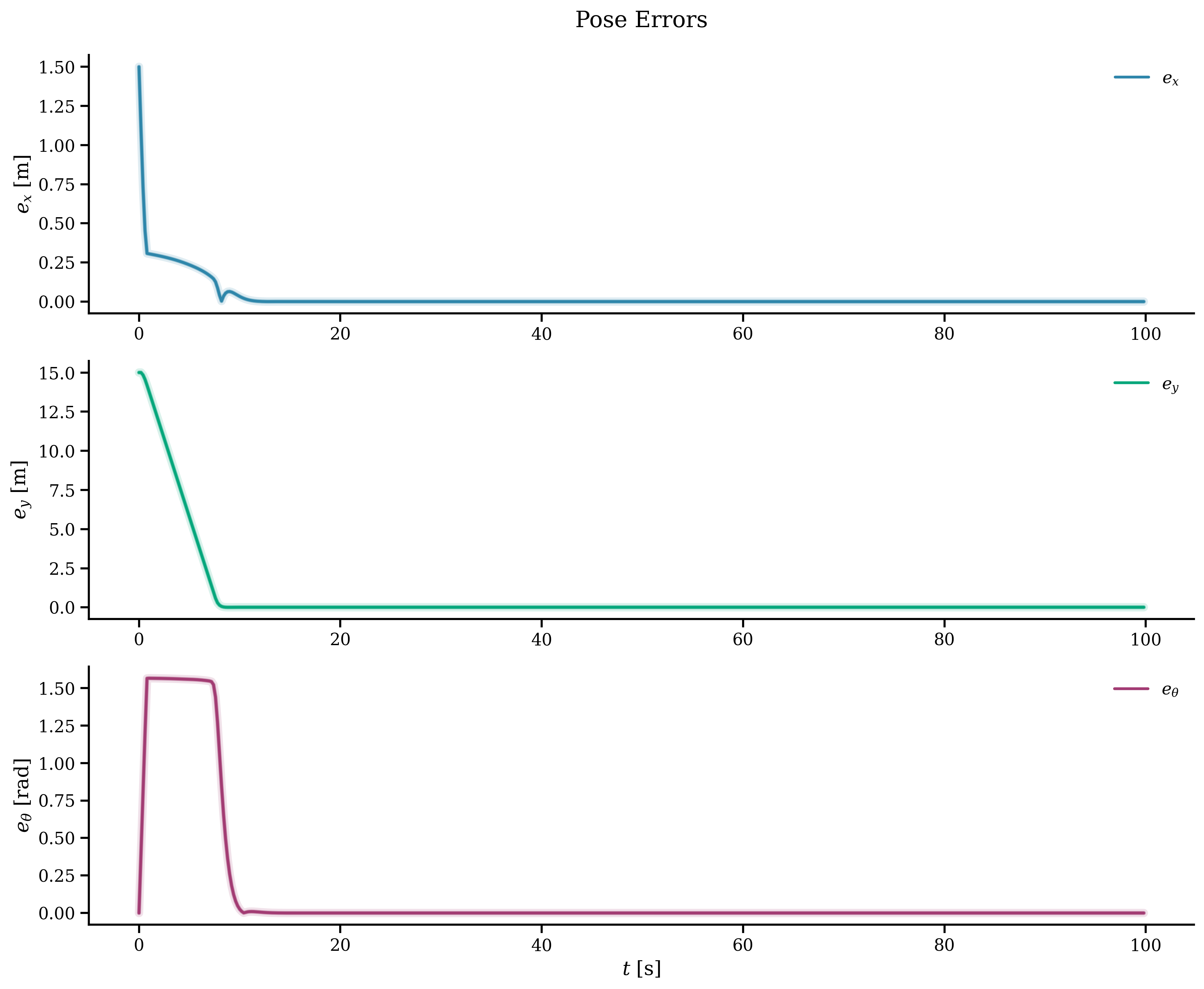
To end this part, we can see the control input and the error. Everything looks to be working great. The control input is even capped at the max value defined in one of our constraints.

Outro

We went through how to create a simple NMPC for a wheeled robot. I’ve also implemented it for a differential-drive kinematics and even to track a trajectory, but it’s essentially the same; you can take a look at it on my GitHub repo. You can plug in your kinematics or dynamics and make it work. Of course, the matrices $Q$ and $R$ may need to be tuned but that’s pretty much it.

Keep in mind this is just a very first approach to an MPC implementation, there are a lot of interesting variants out there that are worth taking a look into.